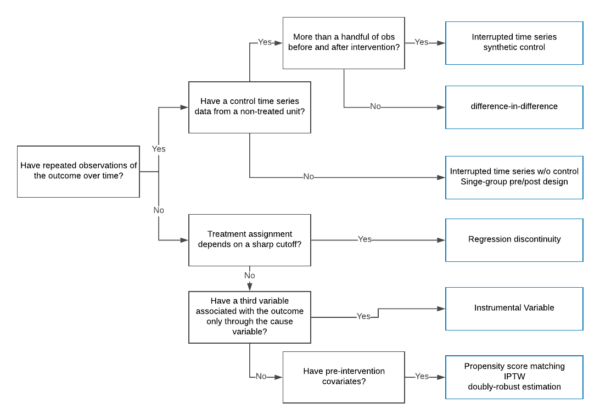
Potential Outcomes and the Fundamental Problem of Causal Inference

Fundamental Problem of Causal Inference

Suppose each individual in a population of interest can be exposed to two alternative states of a cause, i.e. receiving a treatment or not. Each individual has a potential outcome under each treatment state, even though each individual can be observed in only one treatment state at any point in time. The counterfactual, then, is whatever treatment state that the individual is not in at any given time.

The potential outcomes for each individual are defined as the true values of the outcome of interest that would result from exposure to the alternative causal states. The potential outcomes for each individual are y_1i and y_0i for treatment (1) and control (0), respectively. Because y_1i and y_0i both exist theoretically for an individual, an individual causal effect can be thought of as y_1i − y_0i. Because it is impossible to observe both y_1i and y_0i for the same individual at the same time, effects cannot be calculated at the individual level.

Researchers must analyze an observed outcome variable Y that takes on values y_i¹ for treatment group individuals and y_0i for control group individuals, with unobserved counterfactuals y_1i for the control and y_0i for the treatment groups. Average causal effects can be modeled using causal inference techniques if defendable assumptions are met that allow for the estimation of the average unobservable counterfactual for each group.

The fundamental problem of causal inference is that for the treatment group Y₁ is observable but Y₀ is an unobserved counterfactual, while for the control group Y₀ is observed and Y₁ is an unobserved counterfactual. We only have half the information necessary for calculating a causal effect size for any given individual. The observable outcome variable Y can be defined as:
Y = D**Y₁ + (1−D)Y₀

Average Treatment Effects

Since it is impossible to observe individual-level causal effects, causal inference focuses on aggregate causal effects as averages of individual-level effects. The broadest aggregation of treatment effects is the unconditional ATE, which is the difference between the expected outcomes for the treatment and control groups.

• Average Treatment Effect on the Treated (ATT):
  Expected value given one is treated in the sample
  E[Y_1i−Y_0i|D_i=1] = E(Y_1i|D_i=1) − E(Y_0i|D_i=1)

• Average Treatment Effect on the Control (ATC):
  Expected value given one is not treated in the sample
  E[Y_1i−Y_0i|D_i=0] = E(Y_1i|D_i=0) − E(Y_0i|D_i=0)

• Average Treatment Effect (ATE):
  Unconditional expected value (also, ATT+Selection Bias)
  E[Y_1i−Y_0i] = E[Y_1i] − E[Y_0i]

The Stable Unit Treatment Value Assumption (SUTVA)

The assumption that the value of Y for unit u when exposed to treatment t will be the same (1) no matter what mechanism is used to assign treatment t to unit u and (2) no matter what treatment the other units receive. When the SUTVA assumption is met, this allows us to say that the outcome for individual i of treatment d under treatment is y_i1(d) = y_i1 and under control is y_i0(d) = y_i0.

A good example of a SUTVA violation is a vaccine program, in which individuals receive vaccines inside of communities that receive vaccination programs. The individual treatment effect of a vaccine given to a person changes based on the number of vaccines given in her community. When herd immunity is reached, an individual’s vaccine will have no effect, and the treatment effect will be much higher in communities with high disease prevalence as a result of low vaccination rates. The total effect of the vaccine, then, is the combined effect of the vaccine program in the community and the effect of the vaccine on the individual, which may be strongly influenced by herd immunity in the community. The indirect effect of the vaccine program would be the difference between outcomes for an unvaccinated individual in otherwise identical communities with and without a vaccination program.

To conduct an accurate evaluation of a vaccine program, a nested design would be used, in which the assignment of vaccine programs to communities is randomized and vaccination to individuals within the community is also randomized. The experimental evaluation would allow for the total effect to be accurately estimated, but if this were an observational study—that is, in the absence of random assignment and a nested design—the SUTVA assumption would be violated, making causal inference more challenging.

Selection Bias in a Näive Estimator

Comparison of the treated and control units:
\(\\begin{split} E(Y_i\|D=1)-E(Y_i\|D=0) = & E(Y\_{1i}\|D_i=1)-E(Y\_{0i}\|D_i=0)\\\\ & + \\textcolor{red}{\[E(Y\_{0i}\|D_i=1)-E(Y\_{0i}\|D_i=0)\]} \\end{split}\) Where [E(Y_0i|D_i=1)−E(Y_0i|D_i=0)] is the selection bias. This means that we can only eliminate selection bias in cases where E(Y_0i|D_i=1) = E(Y_0i|D_i=0). That is, when the expected observed outcome from the control group under controls is the same as the expected potential outcome that would have occurred had those in the treatment group been exposed to the control condition. Selection bias occurs when systematic differences exist between the group in the treatment condition and the group in the control condition.

A difference in means test requires a full independence assumption.

Regression Control

Linear Regression Review

The standard treatment of regression assumes Y_i = X_iβ + ϵ where X_i is a matrix of coveriates and (for the CNLRM) ϵ_i ∼ N(0,σ_ϵ²I_n) with either X fixed under repeated sampling or $\epsilon \protect\mathpalette{\protect\independenT}{\perp}X$. Under this setup, the best linear unbiased estimator of β is β̂_OLS = (X′X)⁻¹X′y, found by choosing β̂ to minimize the sum of squared residuals Σ_i = 1ⁿ(y_i−X′_iβ̂)². Under the assumed model E[β̂_OLS = β and V(β̂_OL**S) = σ_ϵ²(X′X)⁻¹.

This says nothing of causality. Only about the estimated versus the “true” model. We need the conditional independence assumption (CIA) to establish causality.

Conditional Expectation Function and Regression for Causal Inference

Angrist and Pischke motivate regression somewhat differently.

• Begin with the population (rather than the sample) and focus on the conditional expectation function (CEF) E[Y_i|X_i=x], the population for a fixed value of x.

• The Law of Iterated Expectations (LIE) tells us that E[Y_i] = E[E(Y_i|X_i)]. Say that the population is divided by gender. We could take the conditional expectations by gender and combine them (properly weighted) to get the unconditional expectation. That is, the average of the conditional averages is the unconditional average.

• LIE lets us decompose Y_i into the CEF and “residual”: Y_i = E[Y_i|X_i] + ϵ_i where ϵ_i is mean independent of X_i(E[ϵ_i|X_i]) = 0 and $\epsilon_i {\perp}X_i$

• Any random variable Y_i can be broken into the part “explained by X_i” and an orthogonal residual.

The CEF tells us the population average of Y_i for any given value of X_i. In addition to the decomposition property, there are two notable properties of the CEF:

• CEF Prediction Property: CEF is the minimum mean squared error (MMSE) predictor of Y_i|X_i

• ANOVA Theorem: V(y_i) = V[E(y_i|x_i)] + E[V(y_i|x_i)]

Assumptions in a Regression Control Design

In a simple linear regression, we need four assumptions to identify the causal effect:

• Conditional Mean Independence Assumption: E[Y_1i|D_i = 1, X_i) = E(Y_1i|D_i=0,X_i) and E[Y_0i|D_i = 1, X_i) = E(Y_0i|D_i=0,X_i). The observed mean outcome value for the treatment group should be identical to the counterfactual mean that the controlled units would have taken had they been treated. The observed mean outcome value for the control group should be identical to the counterfactual of the outcome values that the treated units would have taken if they had not been exposed to treatment.
  If the treatment and control groups are systematically different in their respective observed and counterfactual potential outcomes, the mean independence assumption is violated and selection bias will harm inferences.

• Linear Covariate Effects: The underlying model is Y = α + β_iD_i + u_i, where α is an intercept, β_i is the coefficient, and u_i is the population residual. When the treatment variable is categorical and the regression is a saturated model (the model contains all possible values of treatment), this assumption is satisfied.

• Constant Treatment Effects or Stable Unit Treatment Value Assumption (SUTVA): The SUTVA assumption requires that the treatment is the same for every unit and that there is no interference between units.

  • No interference: $Y_{0i},Y_{0j} {\perp}D_j \forall i\neq j$. The treatment of one unit cannot affect other units.

  • Well-defined treatment: D_i = D∀i

• Possible SUTVA violations: influence across units (spatial and network dependency), dilution/concentration effects (prevalent treatments ⇒ increase/decrease of causal effects).

• For instance, in a medical trial, treatments are not stable when the dosages are different among units. The interference occurs either in form of dilution or spatial dependency. Dilution means that the overall frequency of treatments may dilute the causal effects. For instance, when we randomly assign tutoring for a very large number of students, the treated students may put less efforts during tutoring sessions as tutoring is so common that they have little chance to differentiate themselves from the other students. Spatial dependency occurs when a treatment affects the outcome values of the other treated and controlled units. For instance, when a tutored student teaches the controlled students what s/he learned from a tutoring session, it violates the SUTVA assumption.

• Conditional Independence Assumption (CIA): assuming constant treatment effects, we can weaken the ignorability assumption $(Y_{1i},Y_{0i}) \protect\mathpalette{\protect\independenT}{\perp}D_i$ to be conditional on some set of covariates x_i: $(Y_{1i},Y_{0i}) \ind D_i|X_i$

Under (1) independence of treatments and potential outcomes given covariates (CIA), (2) linear separability of covariates, and (3) constant treatment effects, we can use regression to estimate the ATE.

Choosing Covariates and the Bad Control Problem

The assumption that a regression model is “saturated in X_i” means that there is a parameter for every combination of predictor values in the data. This doesn’t work if predictors are continuous, and gets unwieldy quickly, even with discrete predictors. As a result, inference may depend on functional form (linearity) or other assumptions.

We often worry about “confounders”, which are variables that are related to both D and Y variables: D ← X → Y. If X is a confound, then even if there is no true association between D and Y, E[Y_i|D_i=1] ≠ E[Y_i|D_i=0] if we do not take X into account. So we condition on X to “block” this non-causal path of association between D and Y. Causal interpretations of regression can sometimes be justified by assuming “no unmeasured confounders”. Good controls are confounders that we can think of as being fixed at the time the regressor of interest [treatment] was determined..

Bad controls are those which are “themselves outcome variables in the notional experiment at hand,” and which introduce a variant of selection bias. “Colliders” are variables that are included as controls that are caused by D and by Y (D → X ← Y). Bad controls guarantee selection bias. This is very common in the literature. Solution: don’t include post-treatment controls.

The Conditional Mean Independence Assumption is violated when we omit covariates that actually represent systematic differences in the outcome values between the control and treated groups, and when we include post-treatment controls. For instance, when we analyze the effect of car accidents on the cancer rates, we should not control for the rates of hospital admission. Although car accidents itself has no causal effect on the cancer rates, units that are admitted to hospitals with car accidents should have a lower cancer risk than those that are admitted to hospitals without car accidents. Thus, the conditioning on hospital admission creates a systematic difference between the treated and control groups.

Matching

Assumptions in a Matching Design

• Conditional mean independence assumption:
  x_i: $(Y_{1i},Y_{0i}) \protect\mathpalette{\protect\independenT}{\perp}D_i|X_i$
  This assumption states that if X is fixed to specific values, the outcome values should be independent from the treatment assignment. Conditional on X_i, the mean outcome values should be identical whether they are assigned to a treated or control group.

• Common support assumption:
  0 < P**r(D_i=1|X_i) < 1 ∀i
  This means that conditional on X_i there is no deterministic treatment (non-)assignment.

• SUTVA: There should be neither interference nor different meanings in the treatments among the units of analysis.

With these assumptions, we match observations that have the same (or at least similar) values in the covariates and look at their average differences.

Exact Matching

In the exact matching design, we create pairs of observations that have identical values in the covariates. The mean difference of the pairs provides the unbiased estimates of the ATE.

When we cannot easily implement the exact matching, there exist a wide range of matching methods. The distance metrics include the Mahalanobis distance and the propensity score. The matching algorithms include the nearest neighbor, caliper, and radius matching. Computationally-intensive methods such as genetic matching and optimal matching are also available. King and others also propose a way to approximate to the exact matching (coarsened exact matching). The estimates with these methods do not provide unbiased estimates of ATE, ATT, and ATC but typically provide close approximations.

Procedures in a Matching Design

1. Define Xs (using only pretreatment Xs, so it is fine to keep redoing matching until balance is achieved)

2. Define aggregation of Xs and Distance Metric

   • Exact Matching

   • Mahalanobis Distance: Dist*_*i*, *j* = (*X*_*i*−*X*_*j*)′*Σ*′(*X*_*i*−*X*_*j*), where *Sigm**a is a covariance matrix of full observations (for ATE)

   • Genetic Matching: Weighted Mahalanobis distance, Weights are iteratively estimated so as to minimize imbalance

   • Propensity Score:

     • Propensity Score Theorem: Distance metric in ρ = P**r(D=1|X) not in X

     • Absolute PS distance: |ρ_i−ρ_j|

     • Squared PS distance: (ρ_i−ρ_j)²

     • Linear PS distance: |logit(ρ_i)−logit(ρ_j)|

     • (Unlike Mahalanobis distance, these metrics are unidimensional.)

3. Implement Matching Methods:

   • Nearest Neighbor: with or without replacements, assignment rule for ties. Nearest neighbor uses the most similar match. Caliper matching restricts the maximum distance. Radius matching uses all neighbors within the maximum distance.

   • Interval: Classify all observations into “bins” defined for every combination of X; Coarsened exact matching discretizes X and then uses exact matching.

   • Optimal: Computational system for matching that minimizes imbalances.

4. Balance Assessment: assess quality of matching using difference in the mean between matched pairs (re-do parts 1-3 if needed)

5. Estimate average causal effect: calculate average difference between the two groups; regression control with propensity score weighting provides “doubly-robust” regression.

Instrumental Variable

Regression and matching both rely on conditional ignorability (conditional independence) assumptions: that $(Y_{1i},Y_{0i}) \protect\mathpalette{\protect\independenT}{\perp}D_i|X_i$ for some observed covariates X_i. Regression tries to “control away” the effects of other Xs. Matching tries to “balance on” the Xs. Instrumental variable models take a different approach: trying to locate some source of exogenous variation in the causal variable of interest.

An instrumental variable Z is an explanatory variable of D which is only related to Y through D. The instrumental variable approach is a solution to violations of the conditional independence assumption (ommitted variable bias). That is, if a set of X_i variables cannot be found such that $(D_i|X_i) {\perp}\epsilon_i$, but $Z_i {\perp}\epsilon_i$ and Cor**r(X_i,Z_i) ≠ 0, then Z_i is a source of exogenous variation in the causal relationship between D and Y. Through Z’s effect of D it is possible to isolate a part of D that is uncorrelated with ϵ. Because of this, the stronger the correlation between Z and D, the stronger the instrumental variable will be, resulting in more precise estimates of treatment effects.

Assumptions and Properties of the CONSTANT EFFECT DESIGN

1. Non-zero Effect of Instrument on Treatment: Cov(Z_i,D_i) ≠ 0. This ensures that the instrument is useful to predict the assignment of treatments. The higher the covariance, the better.

2. Exclusion Restriction: Z_i is only related to Y_i through D_i. Must be theoretically justified.

3. Linearity: As long as the treatment variable is assumed to be dichotomous, the linear model is saturated. Thus, this assumption is rather trivial.

4. Stable Unit Treatment Variation Assumption (SUTVA): First, the treatments should have the same meanings across individuals. In a medical trial, for instance, the doses should be identical and otherwise the SUTVA is violated. Second, there should not be interference. For example, in an experiment about the effect of tutoring on SAT scores, if we assign tutors for a very larger number of students, students may not think tutoring as distinctive opportunities, and thus they may not make efforts in tutoring sessions to obtain higher SAT scores. As a result, the dilution may weaken the causal effect. Moreover, when a tutored student teaches what s/he has learned in a tutoring session to other students, the spatial interference also biases the estimation.

5. Constant Treatment Effect Assumption: If this assumption is met, then this means that the underlying causal effects should be constant across all individuals. This assumption is usually too demanding. In causal inference methods, we usually assume heterogeneous effects and then estimate the average causal effects. To relax this assumption, we need to follow the heterogeneous effect design.

Under these five assumptions, the Wald estimator is an unbiased estimator of the ATE (assuming a binary instrument):
$\hat{\delta}=\frac{\overline{Y}_{i|Z_i=1)}-\overline{Y}_{i|Z_i=0)}}{\overline{D}_{i|Z_i=1)}-\overline{D}_{i|Z_i=0)}}$
Because we make the constant effect assumption, the Wald Estimator provides an unbiased estimate of the ATE, which is also identical to ATT and ATC. If the constant effect assumption does not hold, then the Wald Estimator provides the Local Average Treatment Effect.

Assumptions and Properties of the HETEROGENEOUS EFFECTS DESIGN

Although the Wald estimator is a global estimator in the constant effect design, this property crucially depends on the constant effect assumption. The heterogeneous effect design relaxes the constant effect assumption, while localizing the causal quantity of interest.

• Linearity (shared with Constant Effect Design)

• SUTVA (shared with Constant Effect Design)

• Non-zero instrument effect (shared with Constant Effect Design): E(D_i│Z_i=1) − E(D_i│Z_i=0) ≠ 0 The instrument is related to the treatment (the stronger the better)

• Mean independence of the instrument from potential outcomes and treatments (“as good as random”)

• Exclusion restriction: the instrument has no effect on Y except through its effect on D. This must be justified theoretically. Violation of the exclusion restriction leads to a biased estimator.

• Monotonicity: D_1i − D_0i ≥ 0∀i or D_1i − D_0i ≤ 0∀i This assumption is often called the no-defiers assumption. In the heterogeneous effect design, there exist four groups of individuals depending on their responses to an instrument. The instrumental variable Z_i can be thought of as an encouragement to take the treatment D_i. “Compliers” are those that take D = 1 when Z = 1 and D = 0 when Z = 0. “Always-takers” are those that always take D = 1, while “never-takers” never take the treatment D = 0. Finally, “defiers” take D = 1 when Z = 0 and D = 0 when Z = 1. The monotonicity assumption states that no defiers exist in the sample. The monotonicity assumption requires that the instrument only affects individuals in one way: it can only “push” units to take the treatment or not, but it can never “pull” them away from treatment.

  • Responses to instrument:

  • Complier: D_{Zi = 1, i} = 1 > D_{Zi = 0, i} = 0 (treatment status is the same as instrument value)

  • Always-taker: D_{Zi = 1, i} = 1 = D_{Zi = 0, i} = 1 (treatment status is irrelevant to instrument value)

  • Never-taker: D_{Zi = 1, i} = 0 = D_{Zi = 0, i} = 0 (treatment status is irrelevant to instrument value)

  • Defier: D_{Zi = 1, i} = 0 < D_{Zi = 0, i} = 1 (treatment status is opposite of instrument value)

Under these assumptions, the Wald estimator is an unbiased estimator of the local average treatment effect (LATE). In essence, the LATE is the average treatment effect for compliers. Thus, in the heterogeneous effect design, the causal estimate is localized to the compliers.

Local Average Treatment Effect (LATE) Theorem:
$LATE=E(Y_{D_i=1,i}-Y_{D_i=0,i}│D_{Z_i=1,i}>D_{Z_i=0,i})=\frac{E(Y_i│Z_i=)-E(Y_i│Z_i=0)}{E(D_i│Z_i=1)-E(D_i│Z_i=0)}$
The LATE is essentially the ATE among Compliers. Always- and never-takers can exist, but we cannot calculate their treatment effects.
LATE* ≠ *ATE*, *ATC*, *AT**T

Two-Stage Least Squares Estimator (2SLS)

There are two reasons to use 2SLS instead of the Wald Estimator: (1) the need for multiple instruments in order to create a strong instrument, and (2) the need to achieve conditional independence of the instrument by using covariates.

Multiple instruments

1. First-stage regression: D_i = α₀ + Z_iα + v_i

2. Second-stage regression: Y_i = β₀ + D̂**β₁ + ϵ_i

   • α̂ gives optimal weights for the multiple instruments

   • β̂_i is the weighted average of causal effects for instrument-specific compliers

   • Note that under the heterogeneous effect design, different instruments lead to estimates on different compliers and thus different results. As a result, the over-identification test is useless in the heterogeneous effect design. (Over-identification test: if different instruments lead to different results, they are not valid.)

Instrumental Variable Analysis with covariates

• Changes in assumptions: Conditional mean independence assumption & Conditional exclusion restriction

1. First-stage regression: D_i = α₀ + Z_iα₁ + X_iα + v_i

2. Second-stage regression: Y_i = β₀ + D̂**β₁ + X_iβ + ϵ_i

   • β̂_i is an estimate of LATE weighted by covariate-specific variance of treatment assignment (regression weighting).

Issues with 2SLS

1. Violations of the exclusion restriction are common, cannot be tested for, and lead to bias and inconsistency.

2. Weak instruments may be so inefficient that they do not justify the improvement in consistency. This occurs because the estimators are leveraging only a small portion of the variation if the instrument is a poor predictor of treatment.

3. Finite-sample bias

   • Problem: The second-stage regression contains a predicted variable D̂_i.

   • Weak instruments may occur due to sample correlations that occur by-chance and that do not exist in the population. Thus, they can lead to large bias. This is more likely to occur when the N is small.

   • Consequence: 2SLS is consistent but biased both in coefficient and standard error estimates

   • Diagnostics: Stock-Yogo critical values (F > 10)

   • Solutions: LIML, Just-identified model (median-unbiased), Reduced-form regression

4. Standard error estimates under heteroskedasticity

   • Solution: GMM estimator

5. Non-Linear Models

   • Problem: Dichotomous outcome and treatment variables

   • Solutions: Bivariate probit

   • Note: Non-linear models provide efficiency and global estimates but with parametric assumptions

Regression Discontinuity Design

The (sharp) RDD method utilizes a comparison between treated and untreated units that are close to the threshold that determines application of that treatment, on a continuous variable. RDD Requires a treatment that is determined by an arbitrary cutoff in a continuous variable, in a way to clearly separate control and treated groups. The main goal is then to compare the outcome variable for units just before and just after the threshold as a way to determine the causal effect of treatment by measuring control and treated units that are similar in everything, except for which side of the threshold they are on.

This logic follows one of a natural experiment, in which treatment is seen as an exogenous factor among those units close to it (in the continuous X variable). Thus, all observable and unobservable factors that could be confounders are assumed to be controlled for in that small group. This gives us confidence that the estimator is not biased by problems that affect other common research methods, such as regression models, because there should be no omitted variables nor misspecifications in the model. Other assumptions, however, are necessary.

In the IV design, the assignment of treatments is a probabilistic function of an instrumental variable. In the (sharp) regression discontinuity design, in contrast, the treatment assignment is determined by an arbitrary threshold.

Assumptions in a Sharp RDD

• Switching or Deterministic application of treatment: D = 1 if X ≥ X₀ and D = 0 if X < 0, with no overlap.

• Smoothness: This means that the observed outcome values around the threshold approximate the outcome values at the threshold. This assumption allows us to compare the treated and controlled units to estimate the causal quantities.

• No manipulation: Units cannot manipulate their position relative to the cutoff (if the income cutoff is $20,000 annually, units cannot work more or fewer hours to get just over or under that amount to self-select into treatment).

• SUTVA

RDD identifies only a localized average treatment effect for units near the cutoff. When these assumptions are met, the difference provides an approximately unbiased estimator for the average causal effect at the threshold (when x = x₀). Like the heterogeneous effect IV design, the estimator of the RDD is localized to x = x₀. The more distant from x = x₀ a unit is, the more likely it is that the estimated treatment effect does not apply to it. There is no assumption of homogeneous effect.

There is a tradeoff between choosing larger and smaller “neighborhoods”, and thus it is advisable to test some different bandwiths to assess how estimates change. Larger neighborhoods provide larger samples and more stable estimates while smaller neighborhoods are less likely to exhibit omitted variable bias.

The RDD estimates a function of the continuous variable X as an explanatory variable of the outcome Y which includes a dummy variable for treatment status D. This does not have to be a linear function and is often polynomial. The equation Y_i = f(x_i) + δ**D_i + ϵ_i is fitted once for each side of x₀. This will give us two functions with a cutoff at x = X₀. The difference in values of Y before and after the cutoff is the localized average treatment effect.

Define the bandwidth to minimize the MSE of δ̂_R**D and apply a kernel to weight observations (weighting those closer to x₀ more). Define f(x_i) to get a good approximation, but avoid overfitting. Then calculate the difference in means for the bandwidth values at D = 0 and D = 1.

The RDD is actually a special case of an IV design, in which the treatment assignment is a deterministic function of an instrument. In fact, the “fuzzy” RDD, in which the treatment assignment is a probabilistic function of a threshold, is degenerated to an IV design. The deterministic treatment assignment reduces the required assumptions and thus strengthen the internal validity of the RDD.

Fuzzy RDD

This type of design is similar to a 2SLS model in the instrumental variable method. It is applied to situations in which the treatment D condition is defined by a continuous variable, but in a probabalistic way so that
P(D=1|X≥x₀) ≠ P(D=1|X<x₀). Under that condition, position just before or after the threshold can be used as an instrumental variable for treatment. The larger the difference, the better, and the stronger the instrument will be. This also results in a local average treatment effect relative only to compliers that are near the cutoff.

Self-selection Problem

The most common violation in RDD is related to self-selection violating the no manipulation and smoothness assumptions. Check if units can manipulate their position close to the threshold with density plots (histogram). If there is a sudden jump with an abnormally small number of observations on one side of the threshold and abnormally high number of observations on the other side of the threshold, then there is a high chance of manipulation.

Check if units within the bandwidth are similar in regard to other observable variables by running regression discontinuity analysis with those variables as outcomes. Large differences will provide evidence against the smoothness assumption.

Fixed Effect Model

Fixed effects are used in panel data analyses (where data has been collected for the same subjects over time) to control for time-invariant covariates for each unit. This has the benefit of controlling for large amounts of unobserved, unobservable, or poorly-measured confounds that remain the same within each unit over time, but that differ between units. Fixed effects can also be used for data with clusters of groups to control for variables that are equal for the whole group. Fixed effects only allow for the estimation of within-group, time-variant effects.
Y_i = β₀ + β₁D_i + β₂X_i + β₃A_i + ϵ_i
In the above model, if $Y_{1i},Y_{0i} \protect\mathpalette{\protect\independenT}{\perp}D_i|X_i,A_i$ and A_i is unobserved, then we cannot estimate unbiased coefficients in the model (particularly β₁, the effect of treatment D_i). However, if we have panel data and the characteristics of A_i are fixed in time, then a Fixed Effects model can be used to control for the unobserved A_i.

Assumptions

1. Gauss-Markov Assumptions

2. Conditional mean independence: D_i is independent of Y_i, conditional on observed X and unobserved A covariates. Treatment is as good as randomly-assigned, conditional on X and A

3. Time-fixed unobserved covariates: The unobserved covariates A_i are fixed in time.

4. Constant Effect

5. Functional form: The linearity assumption, the constant treatment effect assumption, and the saturated X**β assumptions are included in this assumption (very demanding!)

6. SUTVA

When these assumptions are met, the two-way fixed effect model yields a causal estimate:
Y_i, t = λ_t + α_i + X_i, tβ + D_i, tδ + ϵ_i, t

Three Ways of Representation

1. Dummy-variable form: a dummy variable is included for each unit

2. First-difference form: uses the change-in Y, λ, α, X, D, ϵ from t − 1 to t

3. Mean-deviation form: subtracts the mean of Y, λ, α, X, D, ϵ from Y, λ, α, X, D, ϵ

Problems and Limitations

• The variance of the treatment variable is limited to within-unit variance.

• Smaller variance in the treatment variable.

• Fixed effects throws away a lot of information and looks only at variation within each unit over time. This reduces efficiency in order to eliminate bias.

• Assumes homogeneous treatment effect. Cannot use time-invariant covariates with theoretical importance. For example, if we anticipate that men and women will respond differently to treatment, then we cannot both use fixed effects and model this theoretically-important heterogeneous treatment effect between units.

• Adding a dummy for each i eats a lot of degrees of freedom.

Differences-in-Differences

The differences-in-differences method works to identify the effect of a cause with a clear moment in time and that affects some units, but not others.

It is superior to simple comparisons between observed pre- and post-treatment conditions because it uses non-treated units’ variation in the outcome to control for time-varying covariates. Without it, any change would be attributed to treatment only, biasing the estimate.

Compare the original treated group with a control group that remains untreated at both t = 1 (pre-treatment) and t = 2 (post-treatment). The difference between treatment and control at t = 2 minus the difference between treatment and control at t = 1 is the diff-in-diff estimate.

For D_i**t where i=group and t=time, D₁₁ = D₂₁ = D₂₂ = 0 and D₁₂ = 1,
δ = [E(Y₁₂)−E(Y₁₁)] − [E(Y₂₂)−E(Y₂₁)] = [E(Y₁₂)−E(Y₂₂)] − [E(Y₁₁)−E(Y₂₁)]

Assumptions of Diff-in-Diff

• Parallel Trends: Y moves parallel for i = 1 and i = 2 and could continue to do so if i = 1 did not receive treatment. E(Y_{0, i, s, t}│X_i, s, t,t) = λ_t + A_sα + X_i, s, tβ
  E(Y_{1, i, s, t}│X_i, s, t,t) = λ_t + A_sα + X_i, s, tβ + δ
  where i is an indicator of an individual, s is a group indicator for treated and control groups (0 and 1), t is an indicator for time (0 and 1), λ_t is time-varying intercept, A_s is a vector of unobserved group-fixed covariates, X_ist is a vector of observed covariates, and D_i is a treatment variable. This assumption is relatively strong as it requires that the causal effect δ should be constant across observations.
  Note: The linearity assumption, the constant treatment effect assumption, and the saturated X**β assumption are included in this assumption (very demanding!).

• SUTVA: This assumption requires that there is no difference in the meanings of treatment across individuals and that there is no interference among units.

• Conditional Mean Independence: E(ϵ|s,t) = 0 This means that conditional on the observed covariates and time, the outcome variable should be independent of the treatment variable. This assumption, for example, is violated when there exists a relevant covariate that is not included in X_ist (where i is an indicator of an individual, s is a group indicator for treated and control groups (0 and 1), t is an indicator for time (0 and 1)). This would also be violated in Y is a cause of D (e.g. a change in minimum wage laws (treatment) is a response to unemployment levels (both outcome and cause of treatment)).

Under these three assumptions, the difference-in-difference estimator is an unbiased estimator for the ATE. Because the parallel trend assumption includes the constant treatment effect assumption, the DID estimator is also an unbiased estimator for the average treatment effect on the treated (ATT) and the average treatment effect on the controlled (ATC).

Violation of the Parallel Trend Assumption

• Diagnostics 1: Plot of Y_(i,s,t) for each group over the pretreatment periods. If the trends are not parallel, it is discouraging.

• Diagnostics 2: Placebo tests – Conduct the DID analysis with a placebo treatment variable (the timing of treatment is placebo, while the treated units are the same) If there are substantial placebo effects, it is discouraging.

• Diagnostics 3: Inclusion of group-specific time-trend variables. Y_i, s, t = λ_t + α_0, s + α_1, st + X_i, s, tβ + D_s, tδ + ϵ_i, s, t. If the estimate of δ changes after the inclusion of the variable, it is discouraging.

Other Limitations

Diff-in-diff assumes fixed treatment timing.

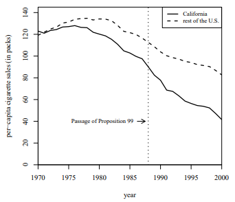
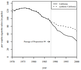
Synthetic Control

The synthetic control design is an extension of the DID design. While in the DID design we condition the outcome variable on its previous values and covariates, the synthetic control design extends the conditioning to all previous outcome values. The synthetic control design produces an unbiased estimate of a causal effect for a single unit.

The synthetic control design “builds” a most-similar control unit to the treated unit to estimate the effect of a cause that has a clear time moment in one particular unit. It can be thought of as a quantitative case study for situations where only one unit was treated. Having the observed Y for D = 0 and t = 1, the synthetic control unit provides a comparable but hypothetical unit for the unobserved potential outcome of D = 0 at t = 2.

Synthetic control makes the assumption of parallel trends more easily believable, leveraging data from several units and several time periods (pre-treatment) to build the artificial version of the unit of interest. It then traces the post-treatment period of that artificial unit, comparing it with the treated unit. The difference between the two in the post-treatment period is the treatment effect.

Time invariant covariates can be included to make the construction of the Synthetic Control respond to factors that the researcer thinks matters. However, the construction of the SC is mostly based on the value of the dependent variable, making it strongly robust due to control for covariates being built into the design.

The weighted average of the control units must be examined to check whtat the synthetic unit is composed of, and if the assumptions hold for that combination of control units. Placebo tests should also be used. Bias of the estimator is bound by a function that approaches zero as the number of pre-treatment periods grows, given perfect matching at outcome and time-invariant covariates.

Assumptions

• Parallel Trends: This holds for post-treatment and can be tested with placebo teststhat fit synthetic control only to arbitrary data to check whether it follows the same trend as the actual unit in pre-treatment

• SUTVA: The SUTVA requires that the meaning of a treatment should be identical across observations and that there is no interference.

• No Pre-Treatment Effect: There should be no effect of anticipation of treatment (no announcement effect) on the treated unit.

• Conditional mean independence assumption: Conditional on the pretreatment outcome variables and covariates, the mean of the outcome variable is independent of the treatment variable. This is a testable assumption. Because neither treated nor control units are treated prior to treatment T₀, E[Y_i**t|Z_i**t,Y_{i, t − 1},…,Y_{i, T0 − 1}] should be similar between treated and control groups during the pretreatment period. The longer the pretreatment period, the better the conditioning.

• Functional form assumption: unlike with FE and DID, the modeling assumptions are more relaxed in synthetic control. The model is saturated, so the linearity assumption is trivial, and there is only one treated unit, so this also makes the constant treatment effect assumption trivial.

Under these assumptions, the synthetic control estimator provides the unbiased estimate of the treatment effect for i = 1. The estimator is the difference between Y for i = 1 and the weighted average of Y of the other units in the posttreatment period. The weight is calculated so as to minimize the differences between Y for i = 1 and the weighted average of Y of the other units at the pretreatment period. The weighted average of Y for control units is called synthetic unit.

Violation of the Conditional Mean Independence Assumption

Problem: Omission of variable that satisfies following conditions:

• Variables are not included in Z_i

• The effects of omitted variables on Y_i, t change after the treatment, OR the omitted variables have effects on Y_i, t only after the treatment

• The changes of the effects are not caused by the treatment

This is essentially omitted variable bias. (For example, if German Unification and a natural disaster occur at roughly the same time and place, then we cannot tell if the effects are from Unification or the natural disaster.)
Potential Solutions: Use a finer temporal scale and/or keep the posttreatment period short.

Other Limitations

Synthetic control allows for only one treated unit and inference is less formal.

Comparisons of Designs

Regression versus Matching

It may not be “fair” to compare a simple linear regression with matching, because the former assumes the unconditional independence of treatment assignment and potential outcomes while the latter is a conditioning strategy. When the unconditional independence assumption does not hold, the estimates of the linear regression are biased but the matching can potentially produce unbiased estimates of the causal effects. When that assumption holds, in contrast, the matching design is degenerated to a simple difference in means, which is identical to the simple linear regression. Thus, the matching design is a generalization of a simple linear regression. Thus, here I compare matching and regression in general.

First, a multiple regression with control variables do not estimate the causal effects such as ATE, ATT, and ATC, while matching produces the estimates of these causal quantities. When causal effects are not constant across individuals, regression coefficients have no causal interpretation in the potential outcome framework. In contrast, the (exact) matching estimator has a direct causal interpretation. Although it is possible to “reweight” a multiple regression and thus generate estimates of the causal quantities (inverse propensity score reweighting design), a multiple linear regression requires these additional steps.

Second, a multiple linear regression is sensitive to the functional form specifications, while matching separates the processes of conditioning and estimation. In a multiple regression, a functional form misspecification of control variables biases the estimates of causal quantities. In contrast, the exact matching does not depend on the functional forms of covariates. Although the propensity score matching depends on the functional forms that produce propensity scores, we can readily use the alternative methods such as the exact coarsened matching.

Third, a linear regression can incorporate multi-valued treatment variables, while matching is largely limited to a conventional dichotomous treatment variables. This point might be a strength of a linear regression. However, a linear regression can include multi-valued treatment variables, exactly because it imposes a functional form about the relationship between the treatment and outcome variables. Thus, the flexibility of a linear regression should be weighted by its functional-form dependency.

Because of these three differences, a linear regression works well when we have strong theory that specifies the functional forms (such as economic models), while matching is useful when we analyze the effect of a dichotomous treatment variable. The regression reweighting design can potentially be as useful as matching. The regression reweighting design is often called doubly-robust; the design is believed to be valid either the assumptions of matching or linear regression hold. Some recent research, however, casts doubt on this claim and demonstrates its sensitivity to functional form specifications. Thus, in practice, people usually report the results both of a matching and regression reweighting designs.

RDD versus DID

First, the conditional mean independence assumption can be tested in the synthetic control method, while it is hard to test that assumption in the RDD. In the synthetic controls, Y conditional pretreatment outcome variables and covariates is different between the treated and control units, the treated and synthetic units should have different Y even in the pretreatment period. Thus, by looking at Y in the pretreatment period, we can see if the conditional mean independence assumption is violated or not.

In contrast, the same logit cannot be applied to the RDD. In the RDD, the outcome variable is conditional on the outcome variable only at t-1. Thus, we cannot make inference about Y at t conditional on Y_t − 1 by looking at Y at t − 1 conditional on Y_t − 2. These two quantities are different, and thus systematic difference in Y_t − 1 conditional on Y_t − 2 between the treated and control units does not mean the systematic difference in Y_t conditional on Y_t − 1 between these two groups, and vice versa.

Second, the DID rests on the constant effect assumption and therefore provide a global estimate, while the synthetic control design does not make such assumption and hence the estimate is confined to a single unit. Unlike other causal inference methods, the synthetic control estimate is not an average treatment effect but it is a treatment effect for i=1. In contrast, the DID can produce the average treatment effect. Thus, the DID has advantage in its external validity. This strength, however, crucially depends on the constant effect assumption. Thus, the advantage in the external validity should be weighted by the plausibility of the constant effect assumption.

Given these differences, the synthetic control method is useful when we are interested in a causal effect of a very unique event, such as the effect of German unification on the economic growth (Abadie and others, 2015), while the DID is useful when we are interested in average causal effects and have strong theory about the functional forms. For instance, in a study about the effect of rainfall on turnout rates in election, we are not interested in the causal effect in a particular district but the average effect of rainfall. Furthermore, although the precipitation itself may not be independent from the potential outcomes (possibly because rainfall correlates with generic climate conditions), the difference in rainfall might be exogenous. Thus, in this case, the DID provides a useful insight about the causal relationship.

RDD versus IV

The RDD is actually a special case of an IV design, in which the treatment assignment is a deterministic function of an instrument. In fact, the “fuzzy” RDD, in which the treatment assignment is a probabilistic function of a threshold, is degenerated to an IV design. The deterministic treatment assignment reduces the required assumptions and thus strengthen the internal validity of the RDD.

Regarding the external validity, both designs usually produce local estimates. The IV estimator is confined to compliers without invoking the constant effect assumption (the constant effect assumption globalizes any local estimator), while the estimators in the RDD is usually limited to specific bandwidth. A recent paper proposes to combine the matching design to globalize the RDD estimators; by conditioning on covariates, x has no relationship with y. As a result, the regression line of y on x becomes a flat horizontal line. This means that we can globalize the estimates within [x0-e, x0+e] to the whole support of x. As far as I know, there is no equivalent method for the IV design. Thus, the RDD might also have strength with respect to the external validity.

Despite of these advantages, the applicability of RDD is limited; there must exist a deterministic treatment assignment. The deterministic assignments often exist in institutionalized politics such as elections and scholarship allocation. Thus, it is not surprising the RDD has predominantly used in the election studies and organization research. In contrast, it is relatively difficult to find arbitral thresholds in un-institutionalized politics. In this case, the IV design has a wider applicability. For instance, agricultural production is not a deterministic function of precipitation, but these two variables should have a tight relationship. Thus, as Miguel did, rainfall might be used as an instrument to estimate the effect of agricultural production on the onset of civil war (though the exclusion restriction might be violated).

In addition, the IV design can incorporate the multi-valued treatment variable, multiple instruments, and control variables. The RDD might also be extended to address these issues, but in general the IV design can more easily address these issues. For instance, Abadie proposes a method that can incorporate multiple instruments and control variables. The method, called Abadie’s kappa, essentially combine the regression reweighting design to the IV design. The flexibility of the IV design might be another reason why the IV has been more widely used than the RDD.

DID and Synthetic Control

First, the conditional mean independence assumption can be tested in the synthetic control method, while it is hard to test that assumption in the RDD. In the synthetic controls, Y conditional pre-treatment outcome variables and covariates is different between the treated and control units, the treated and synthetic units should have different Y even in the pre-treatment period. Thus, by looking at Y in the pre-treatment period, we can see if the conditional mean independence assumption is violated or not.

In contrast, the same logit cannot be applied to the RDD. In the RDD, the outcome variable is conditional on the outcome variable only at t-1. Thus, we cannot make inference about Y at t conditional on Y_t − 1 by looking at Y at t − 1 conditional on Y_t − 2. These two quantities are different, and thus systematic difference in Y_t − 1 conditional on Y_t − 2 between the treated and control units does not mean the systematic difference in Y_t conditional on Y_t − 1 between these two groups, and vice versa.

Second, the DID rests on the constant effect assumption and therefore provide a global estimate, while the synthetic control design does not make such assumption and hence the estimate is confined to a single unit. Unlike other causal inference methods, the synthetic control estimate is not an average treatment effect but it is a treatment effect for i=1. In contrast, the DID can produce the average treatment effect. Thus, the DID has advantage in its external validity. This strength, however, crucially depends on the constant effect assumption. Thus, the advantage in the external validity should be weighted by the plausibility of the constant effect assumption.

Given these differences, the synthetic control method is useful when we are interested in a causal effect of a very unique event, such as the effect of German unification on the economic growth (Abadie and others, 2015), while the DID is useful when we are interested in average causal effects and have strong theory about the functional forms. For instance, in a study about the effect of rainfall on turnout rates in election, we are not interested in the causal effect in a particular district but the average effect of rainfall. Furthermore, although the precipitation itself may not be independent from the potential outcomes (possibly because rainfall correlates with generic climate conditions), the difference in rainfall might be exogenous. Thus, in this case, the DID provides a useful insight about the causal relationship.

Choosing Between Causal Inference Methods

Previous Comp Questions

• “Causal inference is all about filling in the missing potential outcomes.” Discuss this quote beginning by briefly defining the potential outcomes framework. Describe how each of the following methods “fills in” the missing potential outcome, including how the relevant assumptions can be violated and what impact this can have on estimates: matching; differences-in-differences; regression discontinuity. Use examples (real or hypothetical) to aid your explanations.You can assume that your treatment variable of interest is binary. (Spring 2019)

• Explain the potential outcomes framework for reasoning about causality, assuming you have a continuous dependent variable Yi and a binary “treatment” variable Di. When would a simple difference of means E[Y_i|D_i=1]–E[Y_i|D_i=0] provide a good estimate of the effect of Di on Yi? More broadly, describe and contrast the assumptions necessary for valid estimation of a causal effects using each of the following methods: linear regression (with and without covariates), matching, and instrumental variables. (Fall 2018)

• Describe the potential outcomes framework for defining and understanding causality. You can assume a binary treatment variable. Be sure to be clear, concise and formal. What assumptions are necessary to estimate a treatment effect when the treatment is completely randomly assigned? Give an example of a method for estimating a treatment effect when treatment is not truly randomly assigned, i.e.,when the researcher does not directly randomize observations into treatment and control groups. What assumptions are necessary for identifying a causal effect and what causal effect is identified under these assumptions? As part of this explanation give an example (real or hypothetical) of an application of this method. (Spring 2018)

• The regression discontinuity (RD) design is a powerful approach to estimating causal effects, but its applications are limited to specific circumstances. Describe the method in terms of the assumptions it requires, what causal effect it identifies, and the basic ways it is usually implemented. Be sure to note what assumption violation(s) are most worrisome and how potential violations can be investigated. Give an applied example, either from existing research or hypothetical/future research, of RD in which you describe how RD works. (Fall 2017)

• The so-called causal inference revolution in political science has emphasized the importance of careful thought about how best to estimate the effects of a treatment on an outcome variable. But a realistic model of causal effects usually allows for the possibility that the effect of treatment may be different for different observations. Under this setup, there is no single “effect” of treatment — various methods for causal inference estimate different treatment effects, usually some sort of average treatment effect. For each of the methods below, describe what effect is estimated by the method and briefly discuss how to interpret this effect:

  1. Linear Regression: you assume that the model includes both a binary treatment variable and other explanatory variables X, but that it is “fully saturated” in X, i.e., there is a dummy variable included for each possible value of the X’s.

  2. Instrumental Variables Regression: assume a binary treatment and a binary instrument with no other covariates in the model.

  3. Regression Discontinuity Design: assume a sharp RD design using the continuity-based framework.

• How does the potential outcomes framework formally define causality and the (causal) effect of some binary treatment variable on some outcome variable?Define selection bias and describe how it can affect the “naïve” estimator of causal effects, which is calculated as the difference between the average treated and the average untreated value for outcome variable.Discuss two different methods for causal inference, describing how each one overcomes potential selection bias and what causal effect(s) each one estimates. (Fall 2016)

• Choose two of following methods for causal inference: simple linear regression, matching, instrumental variables, difference in differences, regression discontinuity, and synthetic controls. For each method you choose, discuss the assumptions necessary for causal identification and the particular causal effect(s) the method can identify under these assumptions. Briefly contrast the two methods you have chosen, discussing their strengths and weaknesses and the types of situations in which they perform better or worse. (Spring 2016)

Study Guide to Previous Comp Questions

• Offer very clear definitions of:

  • Potential Outcomes

  • The Fundamental Problem of Causal Inference

  • Selection Bias

  • Individual treatment effects versus average treatment effects

  • Local Average Treatment Effect, Average Treatment Effect, Average Treatment Effect on the Treated, Average Treatment Effect on the Control

• For each method:

  • Assumptions necessary for causal identification

  • Common violations of the assumptions and the consequences of the violations

  • Particular causal effects that the method can identify under those assumptions

  • Strengths and weaknesses of method

  • A clear example of the use and abuse of the method